 |||
|||
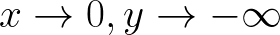
The probability density function of a log-transformed random variable, whose p.d.f was a standard normal
I’ve been working in the log domain over the last couple of weeks, specifically using the natural logarithm, denoted by “ln”. Life has been easier this way.
The dataset I’m working on has a component driven by a random variable X that is distributed normally (a Gaussian distribution) with mean = 0 and standard deviation = 1.
In my last post, I transformed this dataset entirely to the log domain by using the transformation x → ln(x) using numpy and python,
import numpy as np
df_log = np.log(df) # df = my dataframe
In case you missed it, the resulting discussion around this can be found here.
The component that makes up the bulk of the samples in this data is a good old fashioned Gaussian/normal distribution whose probability density function (p.d.f) is given by,
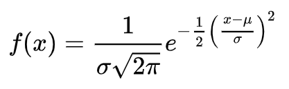 The OG
The mean, mu and standard deviation, sigma are 0 and 1 which gives us the simplest version of the normal distribution, the so-called standard normal distribution,
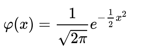 Standard normal distribution
Now, my random variable X has been transformed via the log operator to ln(X). What impact does this have on the distribution of X?
Well, for starters ln(X) represents a transformed random variable and the probability density function associated with the original random variable, X will be transformed into a new probability density function, which will look quite different to its progenitor. This is a crucial point.
So the question becomes, if X is represented by a p.d.f. N(0,1),* then what is the p.d.f of ln(X)?*
If,
then,
There are many ways to answer this question but I used a fairly simple “analytical” approach which I thought would be super useful for anyone going through a similar process (no Taylor expansions here!).
So here goes!
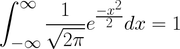
We know that the integral of the p.d.f of X, over its domain = 1. Thus we write,
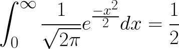
I’m going to consider x > 0 for this derivation, without loss of any generality. Note that half of the area under the p.d.f curve is the integral from 0 to infinity when x > 0 and the other half of the area under the p.d.f curve is obtained when x < 0. This means that for x > 0 and because integrating under the curve is equivalent to finding the area under the curve,
or in more simple terms (1),
Let’s consider the transformation. We need to transform both the variable under which the integration is performed as well as the limits of the integration. Let Y be a new random variable where Y = ln(X). Therefore,
When,
and,
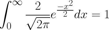
Substituting in (1) above, we get,
Rearranging a bit (2),
(I know, I know, I should have rationalised the denominator, but I’m an engineer doing physics and I don’t want to redo the LaTeX and my python code so maybe let me off the hook please?)
What does this imply? if you look at (2) closely, you’ll notice that the function represented by y integrates to 1 over the entire domain of y. This means that this function must be the p.d.f of y!
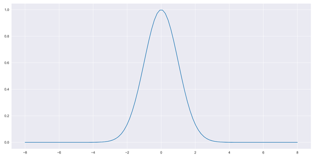
In other words, since Y represents the log-transformed random variable ln(X), the p.d.f of ln(X) must be,
I’ve played around with the notation here and “substituted” y with the symbol x for increased readability giving (3),
That’s a rad looking p.d.f! it’s got exponents e-verywhere! 😂
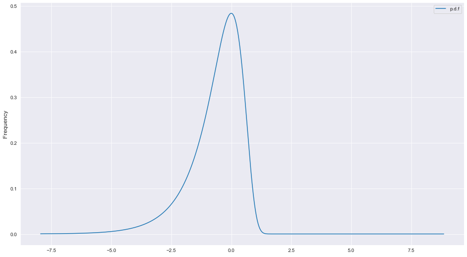
So what does this p.d.f look like when plotted? if the normal distribution looks like a bell curve, what might we expect from (3)?
To answer this question, we turn to python and matplotlib.
import numpy as np
import matplotlib.pyplot as plt
import seaborn as sns #makes plots pretty

x = np.linspace(df_log.min(), df_log.max(), 1000)
#pick any sensible domain here, I'm using the domain of my dataset #for simplicity

f = (2*np.exp(x)/np.sqrt(2*np.pi))*np.exp((-1/2)*np.exp(x)**2)

# this is expression (3) above or the p.d.f of ln(x)
plt.plot(x,f,label='p.d.f')
plt.ylabel('Frequency',fontsize=12)
plt.legend()
And voila!
If anyone is curious, this is the pen and paper version of the derivation above. Note that the pen and paper version is for a more general case of a normal distribution. See you on the next one!
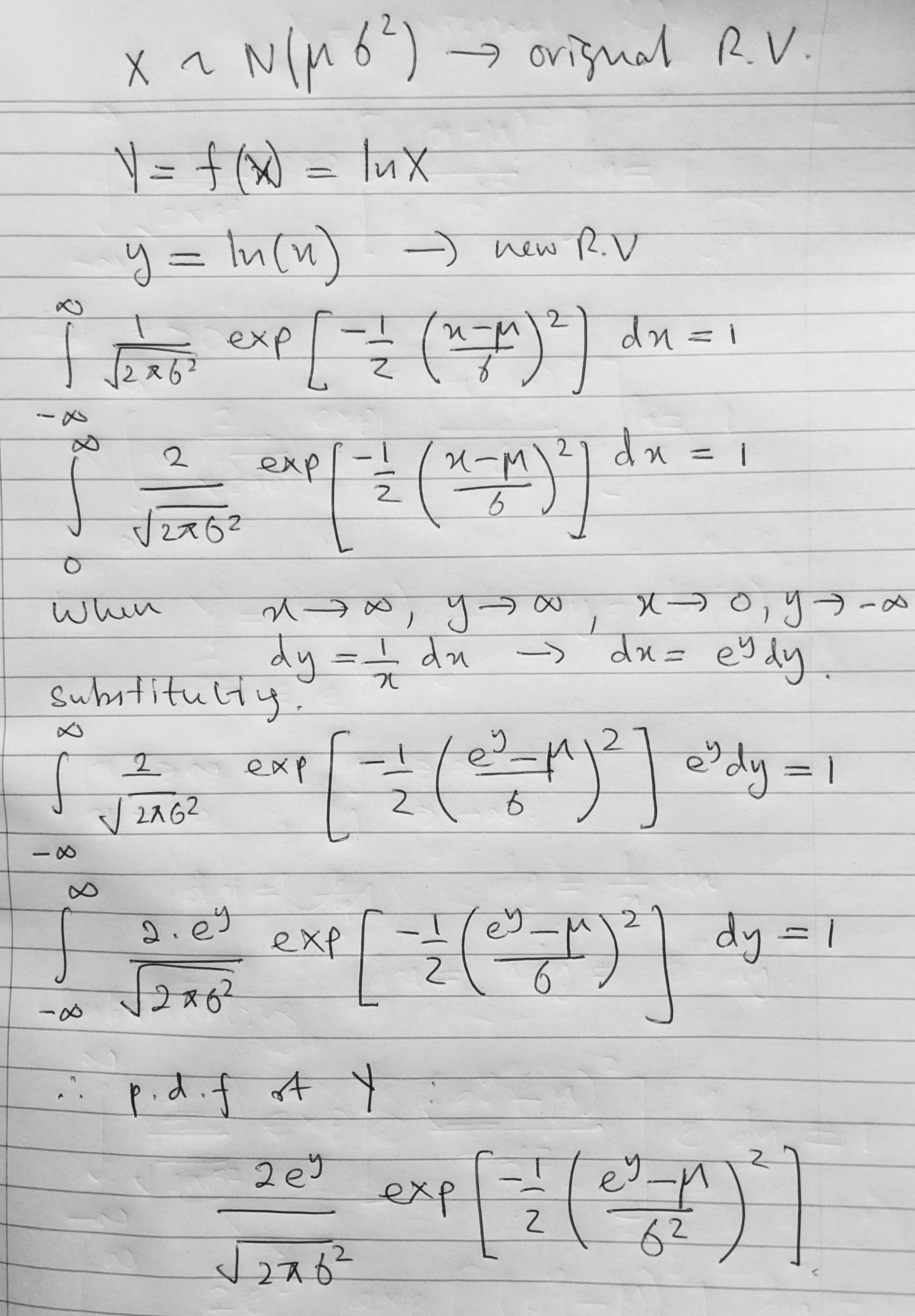 Pen and paper, more general version
Many thanks to Nuzhi Meyen for his insights and Kasun Fernando for spotting an error in my LaTeX.