 |||
|||
How do we choose a reasonable starting point when modeling some data? In the context of statistical inference, this question takes on a prominent dimension as we typically begin our analysis with a fairly simple model that represents the system or process, with reasonable accuracy. This model can then be used to perform a nested sampling operation or equivalent such that we obtain a posterior pdf or estimate.
Often, when building complex models from data, it can be useful to start the process with a least-squares optimized model that fits data obtained from an experiment as a baseline/starting point.
I will consider a fairly straightforward example of instrument data that appears to fit a mixture model comprising three Gaussian distributions and a single Chi-squared distribution. In this example, the choice of these distributions is specific to the domain being considered and can be any mixture of functions relevant to the dataset you may be considering.
The instrument data looks like this,
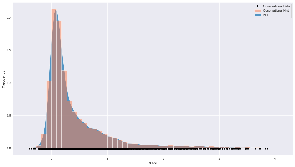 Instrument data
The plot looks quite asymmetric with a long tail beyond 1.5. The black vertical lines along the x-axis are a rug plot that can be instructive in understanding the spread of the data over the x domain.
In this example, we assume that this dataset can be fitted by three Gaussians, which can largely account for the narrow peak just after x = 0 and a Chi-squared distribution (with a degree of freedom value >1) which may be able to account for the long tail beyond x = 1.5. Let’s set this up,
#    f1 = k1*np.exp(-(x-m1)**2 / (2)*(s1)**2)
#    f2 = k2*np.exp(-(x-m2)**2 / (2)*(s2)**2)
#    f3 = k3*np.exp(-(x-m3)**2 / (2)*(s3)**2)
#    f4 = k4*chi2.pdf(x,4,m4,s4)
I’ll be using the least_squares function from scipy.optimize to perform the least squares fitting of this model. This requires setting up the model as follows,
def objective(z):

    y = np.exp(logprob) #instrument data

    k1 = z[0]
    m1 = z[1]
    s1 = z[2]
    k2 = z[3]
    m2 = z[4]
    s2 = z[5]
    k3 = z[6]
    m3 = z[7]
    s3 = z[8]
    k4 = z[9]
    m4 = z[10]


    f1 = k1*np.exp(-(x-m1)**2 / (2)*(s1)**2)
    f2 = k2*np.exp(-(x-m2)**2 / (2)*(s2)**2)
    f3 = k3*np.exp(-(x-m3)**2 / (2)*(s3)**2)
    f4 = k4*chi2.pdf(x,4,m4,s4)


    return y - (f1+f2+f3+f4)
In this context, y is the raw data from the plot above. The objective function thus defined will be subjected to a least-squares minimization that will attempt to reduce the Euclidean distance between y and f1+f2+f3+f4 (the model).
The parameters k1 to m4 will be adjusted by the least_squares function to obtain the lowest distance between the data and the model.
To begin the process, we will need to specify some initial conditions or “best guess” for the parameters k1 through m4 as well as some bounds. I’ve added some reasonable bounds, as well as included where I think k1 through m4 should lie (in order).
initial_values = [1.2, 0.2, 0.1, 0.3, 0.4, 0.1, 0.3, 0.7, 0.2, 0.5, 0.5, 0.5]
bounds=([0,0,0,0,0,0,0,0,0,0,0,0],
        [np.inf,np.inf,np.inf,np.inf,np.inf,np.inf,np.inf,np.inf,np.inf,np.inf,np.inf,np.inf])
The least_squares function in scipy has a number of input parameters and settings you can tweak depending on the performance you need as well as other factors. It may be important to consider the algorithm used by this function to perform the minimization. This may depend on the type of problem you may be working on. It is always useful to check the latest documentation prior to implementation in code. Note the use of a tuple for the bounds variable (a min array and a max array combined to form a tuple).
For my problem, I used the Trust Region Reflective algorithm, which is suitable for large sparse problems with bounds. Calling least_squares,
result = least_squares(objective,initial_values,method='trf',bounds=bounds)I like to write my results into variables so that I may plot the optimized model against the data to visually inspect how closely my model resembles the experimental/instrument data.
k1 = result.x[0]
m1 = result.x[1]
s1 = result.x[2]
k2 = result.x[3]
m2 = result.x[4]
s2 = result.x[5]
k3 = result.x[6]
m3 = result.x[7]
s3 = result.x[8]
k4 = result.x[9]
m4 = result.x[10]
s4 = result.x[11]

f1 = k1*np.exp(-(x-m1)**2 / (2)*(s1)**2)
f2 = k2*np.exp(-(x-m2)**2 / (2)*(s2)**2)
f3 = k3*np.exp(-(x-m3)**2 / (2)*(s3)**2)
f4 = k4*chi2.pdf(x,4,m4,s4)
Plotting the model against the data,
plt.plot(x,f1,label='Component [1]',color='darkorange')
plt.plot(x,f2,label='Component [2]',color='yellow')
plt.plot(x,f3,label='Component [3]',color='green')
plt.plot(x,f4,label='Component [4]',color='red')
plt.plot(x,(f1+f2+f3+f4),label='Combined Components',color='black')
plt.fill_between(x, np.exp(logprob), alpha=0.2, label='KDE')

plt.xlabel('RUWE', fontsize=12)
plt.ylabel('Frequency',fontsize=12)
plt.legend()
Looks like a reasonable fit,
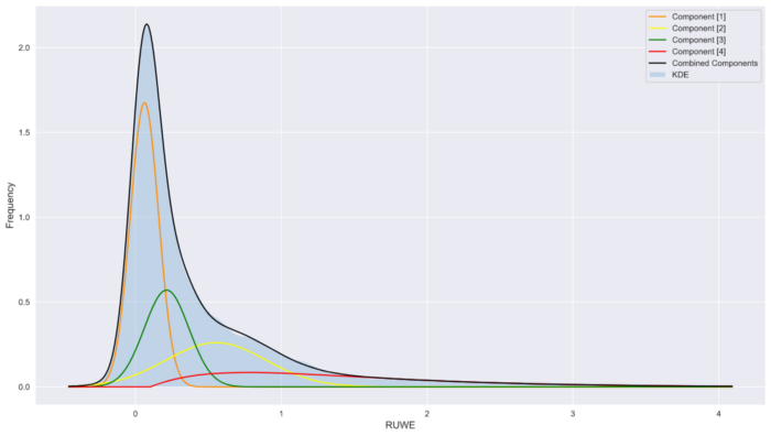 Model vs data
This is a fairly typical workflow for this kind of problem. If the model does not fit the data it is often due to poor model selection or poor selection of initial conditions and bounds (or both!). In the case of poor model selection, it makes sense to go back and examine the context or domain knowledge of the problem in order to suggest a more robust model. In the event of poor initial values and bounds selection, you may need to adjust the values by trial and error until a reasonable fit is achieved.
I hope that this post was instructional. See you on the next one!