 |||
|||
During the last couple of weeks, I’ve been simulating some data for a statistical inference project. While the topic of simulating data is quite broad and depends on the application, I thought that a more general approach of simulating data points that follow a particular probability distribution may be useful to those working on scientific experiments and mathematical modeling.
This post combines a few basic techniques in order to generate some simulated data that follow the distribution of a given probability density function (p.d.f).
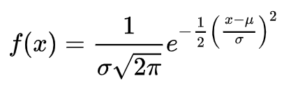
Let’s assume that we have a p.d.f of the form,
def pdf(x):
    F = np.exp(-x**2/2)
    return F
Plotting this to verify,
x = np.linspace(-8,8,100)
plt.plot(x,pdf(x))
The choice of function is arbitrary, I’m using a Gaussian p.d.f here for simplicity/as a toy problem.
The goal now is to generate some simulated data points that follow the same distribution as say, the p.d.f above (or equivalent). Let’s get figure out how to do this!
Inverse transform sampling (ITS)¹ is a robust technique that can generate a set of samples based on a given p.d.f thus delivering a simulated dataset that follows the parent distribution.
ITS involves taking the integral of the given p.d.f and using a fairly intuitive method to generate the required samples.
However, as far as I’m aware, popular Python packages such as SciPy and Numpy do not have an ITS implementation that comes out of the box in the form of a Python class or function.
As an alternative, there are some pretty neat ITS implementations built on SciPy and Numpy. For example, Peter Will’s implementation is great. I’ve tested it out on a few cases over the last couple of weeks and it worked really well for me. Peter’s code is well documented and getting the package set up using his Github repo takes less than five minutes. Peter has also provided a helpful getting started guide in the form of a Jupyter/ipython notebook.
I also came across some great conversations about ITS on Github as well as a feature request to SciPy. Have a look.
If you don’t want to ITS and integrate your way through the problem, here’s a great alternative.
This basically involves generating a large number of random data points in a 2D plane (assuming a 2D problem) on top of the given p.d.f then considering a random data point, checking it’s Y value against the Y value of the p.d.f and storing the corresponding X value if Y(random point) < Y(p.d.f).
Doing this over a set of Y values will generate a set of X values that follow the p.d.f. No integration required!
Let’s implement this in Python.
Let’s begin by specifying our p.d.f. I’m taking a slightly more complicated example for this implementation but again, you can use a p.d.f of choice.
def pdf(x):
  k1 = 120.92391503
  k2 = 74.32971291
  k3 = 10.6030466
  k4 = 6.57300503
  K  = 434.34648701

  f1 = k1*np.exp(-(x-8.16388650e-01)**2 / (2)*(2.55854313e+00)**2)
  f2 = k2*np.exp(-(x-1.03579461e+00)**2 / (2)*(1.14453980e+00)**2)
  f3 = k3*np.exp(-(x-3.15216216e+00)**2 / (2)*(2.99104497e+00)**2)
  f4 = k4*np.exp(-(x-3.72954147e+00)**2 / (2)*(6.86102440e-01)**2)
  F = K*(2*np.exp(x)/np.sqrt(2*np.pi))*np.exp((-1/2)*np.exp(x)**2)
return F+f1+f2+f3+f4
Plotting once again,
x = np.linspace(-10,10,100)
plt.plot(x,pdf(x))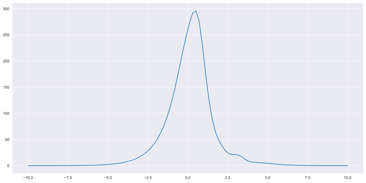
The next step is to generate some random points that can cover the entire grid over which the p.d.f is defined in the plot above.
I found that the Python packageShapely can be leveraged to generate these points given a bounded rectangular region as the grid above. Shapely has polygon objects which can be manipulated to generate points within any shape you can think of! Shapely is available via pip command or Anaconda’s package manager. Importing Shapely and defining the rectangular space (polygon) over which to generate random points,
import numpy as np
from shapely.geometry import Polygon, Point

poly = Polygon([(-10, 0), (10, 0), (10, 400),(-10, 400)])
min_x, min_y, max_x, max_y = poly.bounds
Developing a function that generates random points within this polygon,
def random_points_within(poly, num_points):

    min_x, min_y, max_x, max_y = poly.bounds
    points = []

    while len(points) < num_points:
       random_point = Point([random.uniform(min_x, max_x),  random.uniform(min_y, max_y)])
       if (random_point.within(poly)):
           points.append(random_point)

    return points
Let’s generate 100,000 random points in this space,
points = random_points_within(poly, 100000)
#sampled data points
xs = [point.x for point in points]
ys = [point.y for point in points]
Plotting to verify,
plt.scatter(xs, ys,alpha=0.2, label='Random Data Points')
x = np.linspace(-10,10,100000)
plt.plot(x,pdf(x),color='r',label='PDF')
plt.xlabel('X', fontsize=12)
plt.ylabel('Frequency',fontsize=12)
plt.legend()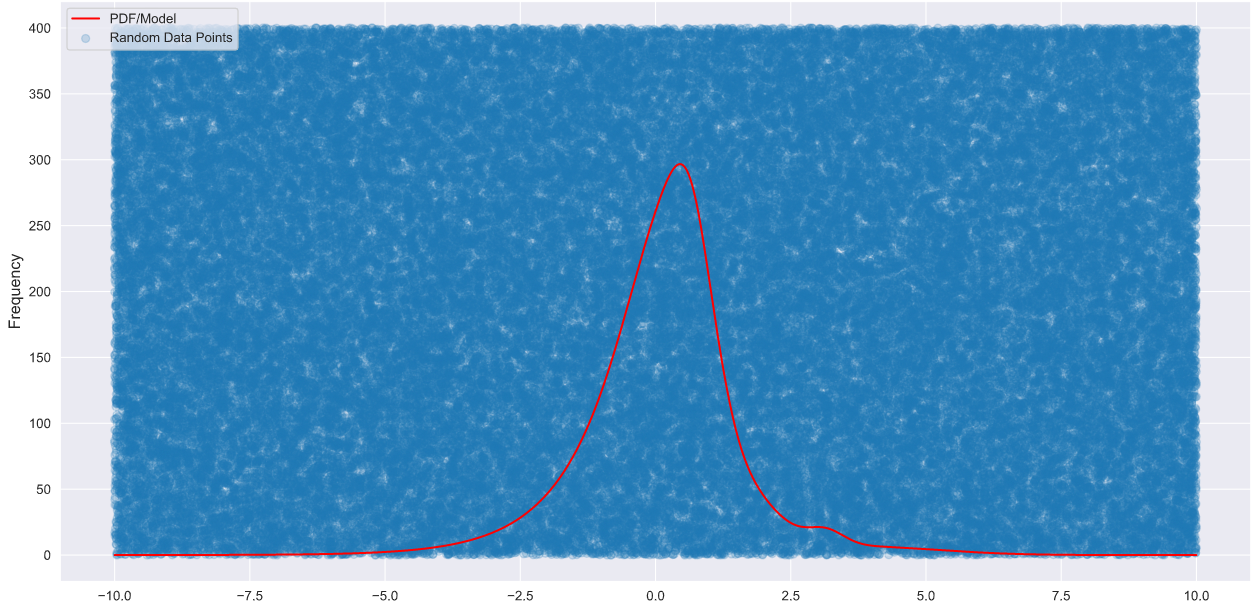
I like to work with data frames so I’m going to implement the core logic that selects the relevant data points using Pandas. Feel feel to use whatever data structure you like at this point,
df = pd.DataFrame({'xs':xs,'ys':ys},index=None)

#using a list
l = []
for i in range(len(df)):
if df.loc[i,'ys']<pdf(df.loc[i,'xs']):
l.append([df.loc[i,'xs']])
under_curve = np.asarray(l)

#plotting the results
plt.hist(under_curve,bins=100,alpha=0.5, label='Simulated Data')
plt.xlabel('X', fontsize=12)
plt.ylabel('Frequency',fontsize=12)
plt.legend()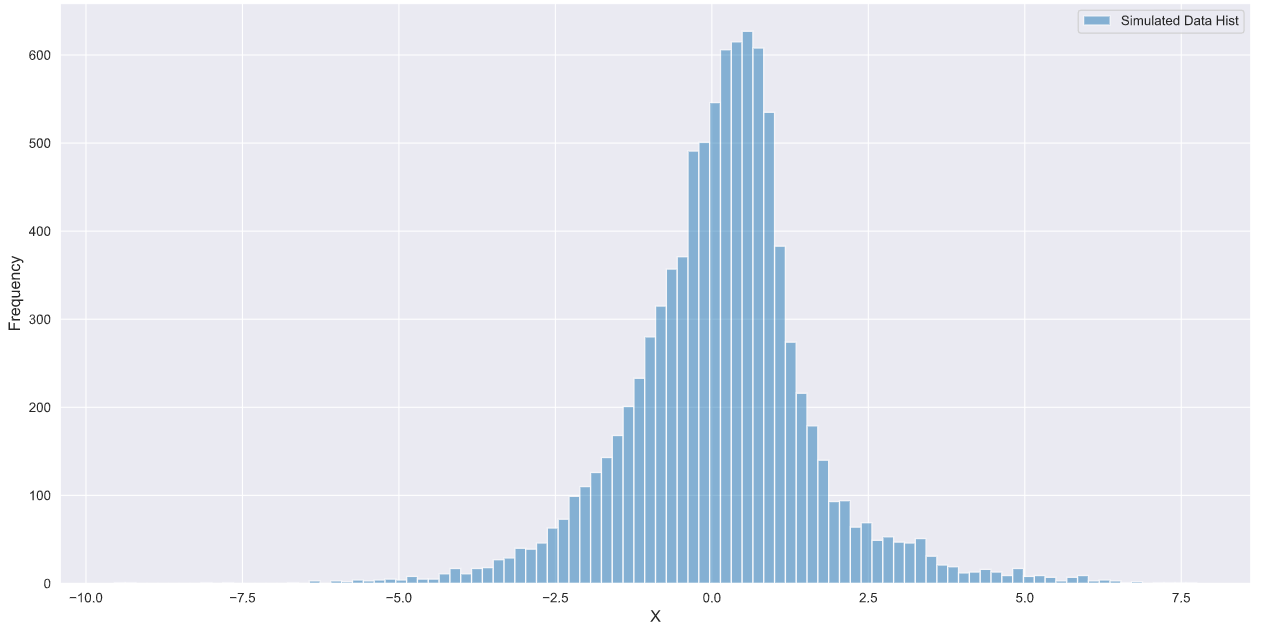
And that’s it! since the points under the p.d.f have the same probability values, the simulated data generated using this method will be consistent with the given p.d.f.
[1] Olver, Sheehan, and Alex Townsend. “Fast inverse transform sampling in one and two dimensions.” arXiv preprint arXiv:1307.1223 (2013).